Skip to section navigation Skip to main content

Which Model Models Best?

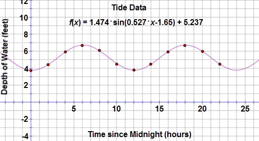
When the sinusoidal function is graphed on the scatter plot, most of the points appear close to the curve.

This graph is a scatter plot displaying the depth of water over the period of twenty-two hours.  The graph is titled ‘Tide Data.’  The horizontal axis is labeled ‘Time since Midnight (hours)’ and extends from negative 3 to 25.  The vertical axis is labeled Depth of Water (feet) and extends from negative 3 to 12.  The graph displays the following ordered pairs:  (0, 3.75), (2, 4.4), (4, 5.9), (6, 6.7), (8, 6.1), (10, 4.5), (12, 3.8), (14, 4.5), (16, 5.9), (18, 6.7), (20, 6), and (22, 4.5).  The curve defined by function f of x = 1.474 times the sine of the quantity 0.527 x minus 1.65 end quantity plus 5.237.

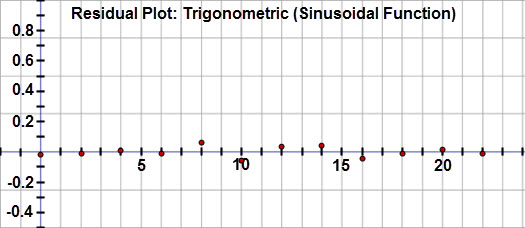
The residual plot reveals that the residuals are random and almost 0, confirming that this function is the best fit for the data.

This graph is a residual plot displaying the residuals for the depth of water over a period of 22 hours when a sinusoidal regression equation (with three iterations) is applied to the data.  The horizontal axis represents the time since midnight and extends from negative 2 to 24.  The vertical axis represents the residual values and extends from negative 0.5 to 1.  The graph displays the following ordered pairs:  (0, negative 1.445), (2, negative 0.822), (4, 0.651), (6, 1.424), (8, 0.797), (10, negative 0.831), (12, negative 1.558), (14, negative 0.885), (16, 0.488), (18, 1.262), (20, 0.535), and (22, negative 0.992).

So, the sinusoidal curve is the best fit for this data.


< Previous Next >