Situation Simulated
 Resources for this lesson:
![]() Key Term
Key Term
Margin of error
You will use your Algebra II Journal ![]() on this page.
on this page.
> Glossary ![]()
> Calculator Resources ![]()
> Teacher Resources: Instructional Notes ![]()
Here are the results of Justyce and Khalid’s simulation for the Blackbirds’ scenario. Items outlined in a blue square highlight the home runs that resulted from the simulation.
Trial |
Trial Results |
Homerun? |
Trial |
Trial Results |
Homerun? |
|---|---|---|---|---|---|
1 |
35 4 3 19 2 29 34 26 33 |
No |
11 |
27 19 7 34 12 26 29 7 29 |
No |
2 |
26 4 2 27 19 11 32 22 34 |
No |
12 |
10 24 2 13 15 9 24 15 17 |
No |
3 |
17 6 10 22 18 23 8 22 21 |
No |
13 |
13 6 29 3 15 29 9 23 22 |
No |
4 |
8 34 34 27 5 4 16 28 30 |
No |
14 |
3 34 28 24 33 24 22 16 24 |
No |
5 |
25 5 28 25 3 16 1 16 26 |
Yes (1) |
15 |
23 27 12 5 30 22 8 32 17 |
No |
6 |
12 3 29 20 11 17 7 31 25 |
No |
16 |
1 22 25 2 6 7 26 12 12 |
Yes (1) |
7 |
34 17 12 25 30 19 26 29 26 |
No |
17 |
16 8 34 28 4 15 7 2 13 |
No |
8 |
20 35 19 6 3 34 26 27 25 |
No |
18 |
31 10 1 1 21 16 35 3 10 |
Yes (2) |
9 |
27 1 15 15 25 17 17 26 35 |
Yes (1) |
19 |
10 29 3 11 1 19 9 21 35 |
Yes (1) |
10 |
14 29 18 22 25 6 33 17 20 |
No |
20 |
28 5 25 6 3 9 7 4 28 |
No |
For Justyce and Khalid, they had 5 out of 20 games resulting in a home run. Out of a total of 180 hits (20 games with 9 hits), they had 6 home runs. That is, they saw a 6 in 180, or 1 in 30, chance of getting a home run. Compare this to the original stated average of a 1 in 35 chance of getting a home run. Khalid and Justyce’s results very closely model this average.
The more trials we conduct, the closer we should see the average approach this 1 in 35.
 Algebra II Journal: Reflection 3
For Justyce and Khalid, they had 5 out of 20 games resulting in a home run. Out of a total of 180 hits (20 games with 9 hits), they had 6 home runs. That is, they saw a 6 in 180, or 1 in 30, chance of getting a home run. Compare this to the original stated average of a 1 in 35 chance of getting a home run. Khalid and Justyce’s results very closely model this average.
The more trials we conduct, the closer we should see the average approach this 1 in 35.
Using the graph in your Algebra II Journal ![]() , add a dot for your simulation. (Be sure to convert your mean to be out of 180.)
, add a dot for your simulation. (Be sure to convert your mean to be out of 180.)
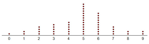
Chance of Home run (chance in 180)
The results of 50 simulations should look very familiar to you! This is approximately a normal curve. The sample mean of this data is 5. Thus, based on the simulations, there is a 5 in 180, or a 1 in 36, chance of a batter getting a home run when he gets a hit.
WOW! This sample is really close to the original population statistic given by Justyce’s mother, who says that a player has a 1 in 35 chance of hitting a home run.
What this shows is that the more trials you perform, the closer your results will approach the actual population mean. However, this plot shows us much, much more. Recall the 68-95-99.7 Rule, which states that 95% of the data should be centered about the mean. For our sample data, this means that 95% of the data centers around the sample mean 5. Remember, according to the 68-95-99.7 Rule, 95% of the data falls within two standard deviations above or below the mean. For this simulation, the standard deviation is (approximately) 1.5, so two standard deviations is (approximately) 3. Therefore, 95% of the data falls between 2 and 8.
What does this mean? It is important to remember that the simulation is producing sample data. We can compare the sample mean and standard deviation to the population mean. We saw the sample mean of 1 in 36 was very close to the population mean of 1 in 35. There is some error in our sample data. The standard deviation gives us a margin of error. Here is how we can interpret our sample data:
A batter has a 5 in 180 chance of hitting a home run, ± 3 in 180.
Simplifying the fractions here, we can state:
A batter has a 1 in 36 chance of hitting a home run, ± 1 in 60.
Or if we express each ratio as a decimal we get:
A batter has a 0.0278 chance of hitting a home run, ± 0.0167.
The ± 3 in180, or ± 1 in 60, or ± 0.0167, came from the two standard deviations of 1.5 which equals 3. This “± 0.0167” is the margin of error. It allows us to say with confidence that we can expect the chance of a home run to be about 1 in 36 from our sample set of data, which converts to the decimal 0.0278, with an allowance of ± 0.0167 error. (This number, ± 0.0167, comes from the fact that 95% of the data falls within two standard deviations of the mean, and in this case the standard deviation was 1.5, so two standard deviations was 3 and the simulation was based on 180 hits; 3 divided by 180 equals 0.0167.)
So what exactly is margin of error? Have you ever heard someone say, “I promise to meet you after school at 3:00, give or take 15 minutes.”? If they arrive at 3:10, did they keep their promise? YES! If they arrive at 2:58, did they keep their promise? YES! That “give or take” is the margin of error.
 Back to the baseball example, we can say a batter has a 0.0278 chance of hitting a home run when he gets a hit, give or take 0.0167. With that “give or take” we are within 95% of the data, so we are making a confident statement.