Exploring Other Function Models
 Resources for this lesson:
> Glossary ![]()
> Calculator Resources ![]()
> Teacher Resources: Instructional Notes ![]()
Test and Confirm
Khalid graphs the quadratic regression equation with the scatter plot data, as seen below.
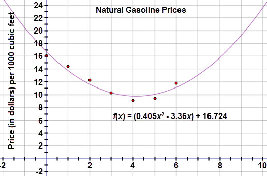
 Khalid: From the graph, it looks like a quadratic model is a good fit. But, I still need to check the residuals and examine the residual plot.
Khalid needs to verify that a quadratic model is the most appropriate model for this data set. To do this he will need to analyze the residual plot to verify that the residuals are small and the plot does not reveal a pattern. If the residual plot is not ideal, he will need to examine other potential models to see if there may be a better fit.
Using your graphing calculator, graph the residual plot. When ready, move to the next page.