A Good Enough Fit?
 Resources for this lesson:
> Glossary ![]()
> Calculator Resources ![]()
> Teacher Resources: Instructional Notes ![]()
 The residual values will have a sum of approximately 0. When analyzing residuals, you want residuals to be as small as possible. The smaller the residuals, the closer the line (or curve) is to the actual values.
It is important to also examine the residual plot. You can find and analyze residuals with your graphing calculator, graphing applet or the Shodor Applet ![]() .
.
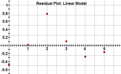
Andrew plots the residuals for the linear model and sees the following:

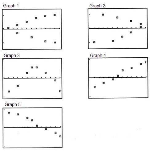
On the residual plot, the points should appear to be randomly dispersed around a horizontal axis. If a pattern emerges from the plot, this is an indication that the model selected may not be a best fit for the data.
In the residual plot for winning times, the data is fairly small and fairly random. This indicates that a line may be the best association for this data set.
Here are some samples of residuals plots that are not random:

 Real-Life Scenarios
> Text version for Real-Life Scenario ![]()
Andrew must also examine the correlation coefficient before making a final decision about the strength of the model.


