Exploring Other Function Models
 Resources for this lesson:
> Glossary ![]()
> Calculator Resources ![]()
> Teacher Resources: Instructional Notes ![]()
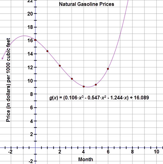
 Khalid graphs the cubic model on the scatter plot. He sees that the model appears to pass through most of the points. This fit appears to be significantly better than the quadratic model. To make sure this is in fact the best fit, he needs to examine the residuals.
Create and analyze the residual plot using your graphing calculator.
When ready, move to the next page.