Exploring Other Function Models
 Resources for this lesson:
> Glossary ![]()
> Calculator Resources ![]()
> Teacher Resources: Instructional Notes ![]()
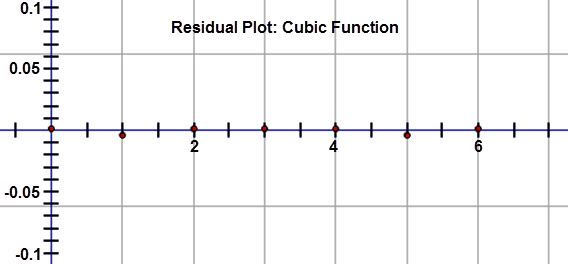
After inspecting the residuals, Khalid notices that the residuals are very close to zero and do not show a pattern. So, a cubic regression is an excellent fit for the data set.
Just to be sure, he decides to calculate a quartic regression. Here is the quartic regression equation:

 Khalid: For this regression equation, the leading coefficient is close to 0. When this happens for a polynomial function, it indicates that the best fit is one degree less. So, the cubic function is in fact the best fit for the data.